What Five Factors Can Affect Giving Meaning to a Traffic Scene

---

final report

Traffic Congestion and Reliability:
Trends and Avant-garde Strategies for Congestion Mitigation

---

2.0 The Nature of Traffic Congestion and Reliability: Causes, How They Are Measured, and Why They Matter

two.one WHAT IS CONGESTION?

Congestion is relatively like shooting fish in a barrel to recognize—roads filled with cars, trucks, and buses, sidewalks filled with pedestrians. The definitions of the term congestion mention such words as "clog," "impede," and "excessive fullness." For anyone who has ever sat in congested traffic, those words should sound familiar. In the transportation realm, congestion normally relates to an excess of vehicles on a portion of roadway at a particular time resulting in speeds that are slower—sometimes much slower—than normal or "free menstruation" speeds. Congestion often means stopped or stop-and-go traffic. The rest of this chapter is devoted to describing congestion and how we measure it, as well as its causes and consequences.

2.2 CAUSES OF CONGESTION AND UNRELIABLE TRAVEL

2.2.1 Background: The Seven Sources of Congestion

Previous work has shown that congestion is the result of seven root causes, often interacting with one another.^five These "seven sources" tin be grouped into three broad categories, every bit shown below:

Category 1 — Traffic-Influencing Events

1. Traffic Incidents – Are events that disrupt the normal menstruation of traffic, ordinarily by concrete impedance in the travel lanes. Events such as vehicular crashes, breakdowns, and debris in travel lanes are the most mutual form of incidents. In addition to blocking travel lanes physically, events that occur on the shoulder or roadside can also influence traffic menstruum by distracting drivers, leading to changes in commuter behavior and ultimately degrading the quality of traffic flow. Even incidents off of the roadway (a fire in a building side by side to a highway) can exist considered traffic incidents if they bear on travel in the travel lanes.
2. Work Zones – Are structure activities on the roadway that effect in physical changes to the highway environment. These changes may include a reduction in the number or width of travel lanes, lane "shifts," lane diversions, reduction, or elimination of shoulders, and even temporary roadway closures. Delays acquired by work zones have been cited by travelers as one of the virtually frustrating conditions they see on trips.
3. Atmospheric condition – Environmental weather can lead to changes in commuter behavior that affect traffic menses. Due to reduced visibility, drivers will usually lower their speeds and increase their headways when precipitation, bright sunlight on the horizon, fog, or smoke are present. Wet, snowy, or icy roadway surface conditions will also lead to the same effect even after precipitation has concluded.

Category 2 — Traffic Demand

1. Fluctuations in Normal Traffic – Day-to-day variability in demand leads to some days with higher traffic volumes than others. Varying demand volumes superimposed on a system with fixed capacity likewise results in variable (i.e., unreliable) travel times, even without any Category 1 events occurring.
2. Special Events – Are a special case of demand fluctuations where traffic flow in the vicinity of the consequence will exist radically unlike from "typical" patterns. Special events occasionally cause "surges" in traffic need that overwhelm the system.

Category iii — Concrete Highway Features

1. Traffic Command Devices – Intermittent disruption of traffic menstruation by control devices such as railroad form crossings and poorly timed signals also contribute to congestion and travel time variability.
2. Physical Bottlenecks ("Chapters") – Transportation engineers accept long studied and addressed the concrete capacity of roadways—the maximum amount of traffic capable of existence handled by a given highway section. Capacity is determined by a number of factors: the number and width of lanes and shoulders; merge areas at interchanges; and roadway alignment (grades and curves). Price booths may also be idea of as a special case of bottlenecks considering they restrict the concrete menses of traffic. At that place is also a wild card in the mix of what determines capacity—driver beliefs. Enquiry has shown that drivers familiar with routinely congested roadways space themselves closer together than drivers on less congested roadways. This leads to an increment in the corporeality of traffic that can exist handled.

Highlight Box 1 discusses how the seven sources of congestion are related to the underlying traffic flow characteristics that create a disruption in traffic. Nosotros typically think of a bottleneck as a physical restriction on capacity (Category 3 in a higher place). Nevertheless, disorderly vehicle maneuvers caused by events have a similar effect on traffic flow as restricted physical chapters.

Because the traffic flow effects are similar, traffic disruptions of all types can be thought of as producing losses in highway chapters, at least temporarily. In the past, the primary focus of congestion responses was oriented to calculation more than physical capacity: changing highway alignment, adding more than lanes (including turning lanes at signals), and improving merging and weaving areas at interchanges. But addressing the "temporary losses in capacity" from other sources is as important.

Highlight Box 1 – What Causes Breakdowns in Traffic Flow?

What causes traffic period to suspension down to stop-and-get weather? The layman's definition of congestion every bit "too many cars trying to use a highway at the same fourth dimension" is essentially correct. Transportation engineers formalize this idea as capacity—the ability to move vehicles past a bespeak over a given bridge of fourth dimension. When the chapters of a highway section is exceeded, traffic flow breaks downwardly, speeds drop, and vehicles crowd together. These actions cause traffic to back up behind the disruption. And then, what situations would cause the overload that leads to traffic backups?

Basically, there are iii types of traffic flow behavior that will cause traffic flow to break downwardly:

1. "Bunching" of vehicles every bit a consequence of reduced speed. As vehicles are forced to get closer and closer together, abrupt speed changes can crusade shock waves to class in the traffic stream, rippling backward and causing even more than vehicles to tedious downwards. Several things tin can crusade vehicles to slow down while traveling in their intended lanes:
   • Visual Effects on Drivers. Driver behavior is a very important part of traffic period. When traffic volume is loftier and vehicles are moving at relatively high speeds, it may take only the sudden slowing downwards of one commuter to disrupt traffic period. Driver behavior in this case is influenced past some sort of a visual cue and can include:
     1. Roadside distractions – unusual or atypical events that cause drivers to become distracted from driving.
     2. Limited lateral clearance – drivers will usually slow down in areas where barriers become too shut to travel lanes or if a vehicle has broken downwardly on the shoulder.
     3. Traffic incident "rubbernecking" – call it morbid curiosity, but most drivers volition slow down just to become a glimpse of a crash scene, even when the crash has occurred in the opposite management of travel or in that location is plenty of clearance with the travel lane.
     4. Inclement weather – poor visibility and slippery road surfaces cause drivers to slow downward.
   • Abrupt Changes in Highway Alignment. Sharp curves and hills can cause drivers to deadening down either because of safety concerns or considering their vehicles cannot maintain speed on upgrades. Another example of this type of bottleneck is in work zones where lanes may be redirected or "shifted" during construction.
2. Intended Interruption to Traffic Period. "Bottlenecks on purpose" are sometimes necessary in guild to manage flow. Traffic signals, freeway ramp meters, and tollbooths are all examples of this type of clogging.
3. Vehicle Merging Maneuvers. This form of traffic disruption has the nearly severe effect on traffic flow, with the exception of really bad weather (snow, ice, dense fog). These disruptions in traffic flow are acquired by some sort of concrete brake or blockage of the road, which in turn causes vehicles to merge into other lanes of traffic. How severely this type of disruption influences traffic flow is related to how many vehicles must merge in a given infinite over a given time. These disruptions include:
   • Areas where one or more than traffic lanes are lost – a "lane-drib" which sometimes occurs at bridge crossings and in work zones.
   • Lane-blocking traffic incidents.
   • Areas where traffic must merge across several lanes to admission entry and leave points (called "weaving areas").
   • State highway on-ramps – merging areas where traffic from local streets can join a freeway.
   • Freeway-to-freeway interchanges – a special case of on-ramps where flow from 1 freeway is directed to some other. These are typically the most astringent class of physical bottlenecks considering of the high traffic volumes involved.

Influencing all of these disruptions in traffic flow is the level of traffic that attempts to utilize the roadway. High need for highway apply—such equally that caused by special events—can compound the bug acquired by disruptions to traffic flow.

2.ii.two How the Vii Sources Crusade Congestion

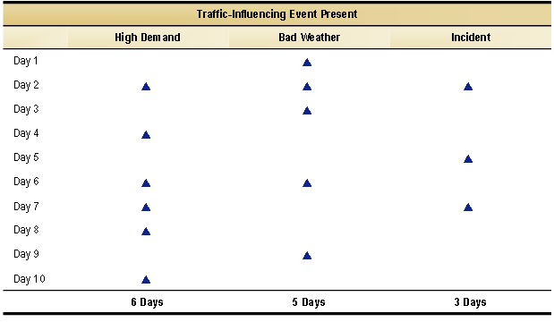
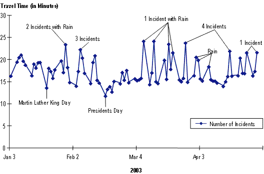
Congestion results from ane—or the interaction of several—of the seven sources on the highway organisation. The interaction tin exist circuitous and varies profoundly from mean solar day-to-24-hour interval and highway-to-highway. The problem is that with the exception of the physical bottlenecks, the sources of congestion occur with maddening irregularity—nothing is e'er the aforementioned from one 24-hour interval to the side by side! Ane twenty-four hours commuters might face up low traffic volumes, no traffic incidents, and practiced weather; the next mean solar day traffic might be heavier than normal, it might exist raining, and a severe crash may occur that blocks traffic lanes. An analysis of how the combination of these events conspires to brand congestion was washed in Washington, D.C. (Table 2.1). The worst traffic days experienced in Washington can be explained past the occurrence and combination of different events.

Another case of the irregularity in event occurrence tin can be seen in the frequency and duration of traffic incidents. Effigy 2.ane shows how traffic incidents occurred on a fourteen-mile stretch of Interstate 405 in Seattle, Washington during peak travel periods for the offset four months of 2003. Some days are relatively incident-free while others have numerous traffic incidents. Interestingly, at least one traffic incident occurred every day during the peaks on this highway. And so, while some days are amend than others, traffic incidents are an unavoidable fact on crowded urban freeways.

Some other source of variability is traffic need, which is rarely the same from day-to-day. On routes heavily used for commuting, weekday traffic is typically much higher than weekend traffic. (On routes in recreational, tourist, or shopping-dominated areas, weekend traffic higher.) Figure 2.2 shows this variability in dramatic way for Detroit freeways. Information technology also shows that there is some variability on weekdays: Thursdays and Fridays are typically the highest traffic days for this catamenia.

The congestion and travel fourth dimension variability caused by planned special events are becoming a major concern for transportation agencies. In a recent survey of state Departments of Transportation (DOTs) by the American Association of Expressway and Transportation Officials and the American Highway Users Alliance, special events were cited as significant contributors to noncommuter congestion. These events may be categorized as:

• Major Sporting Events – This includes sports events within cities (eastward.g., major league baseball, professional football games) and college sporting events in relatively minor academy towns, especially college football. In fact, many higher football games are attended past 100,000 spectators or more, and the associated congestion in towns and small cities (e.g., Ann Arbor, Michigan; Knoxville, Tennessee; and Lincoln, Nebraska) can overwhelm the local highway system on game days. The merely saving grace is that usually there are no more than than seven home games per yr; even so, congestion is significant on these days, requiring a lot of planning and active management by transportation and enforcement personnel.

Table 2.1 Factors Contributing to Extreme Congestion
Ten Worst Days of Washington, D.C. Traffic

Source: Vasudevan, Meenakshy; Wunderlich, Karl East., Shah, Vaisshali; and Larkin, James, Effectiveness of Advanced Traveler Information Systems (ATIS) Under Extreme Congestion: Findings from a Washington, D.C., Case Study, proceedings of ITS America, 2004.

The events that impede traffic menstruation and cause travel to be unreliable often occur in combination. This diagram shows the number of days when different combinations of events occurred during the written report period. For instance, there were three days when incidents occurred—on two of these days only incidents occurred and on 1 twenty-four hours, incidents occurred in combination with high need and bad weather. Equally most commuters know, "some days are worse than others." Pile high demand (say, a Friday before a 3-solar day weekend) on acme of heavy pelting and a lane-blocking crash, and you've got the ingredients for severe congestion.

Figure 2.1 The Number and Elapsing of Incidents Varies Profoundly from Solar day to Day
I-405 Southbound, Seattle, Washington

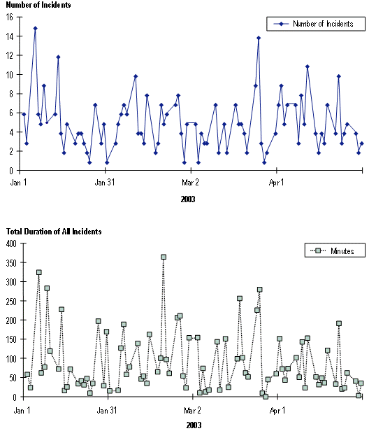
Note: Information shown are for the morning and afternoon peak periods (7:00-x:00 a.m. and iv:00-7:00 p.thousand.) for the period from Jan 1, 2003 to Apr thirty, 2003. Traffic incidents occur in a fairly erratic pattern from day-to-twenty-four hours. Also, how long they last and how many lanes they cake are fairly unpredictable. This erratic behavior contributes significantly to making travel unreliable for travelers.

Figure 2.2 Traffic Levels Vary Substantially over the Course of a Week
Detroit Freeways, 3/11/2001 - four/vii/2001

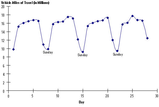
Note: VMT (or "vehicle-miles of travel") is a mutual measure of highway usage. It is calculated as the number of vehicles using the arrangement times the distance they travel. For the time period displayed, Sundays are the low points on the graph. Weekday travel tin can be more than than sixty percent college than Dominicus travel. On weekdays, the tendency toward highway travel later in the week (Thursdays and Fridays) is common in virtually urban areas. While commuting trips are relatively stable throughout the week, discretionary trips are college as the weekend approaches.

• Auto and Horse Races – The rising in the popularity of NASCAR has led to increased congestion effectually race events.
• University "Movement-in Mean solar day" – Several DOTs indicated that the starting time of fall term on college campuses create a surge in traffic for two to iii days. This seems to be a problem in the smaller towns and cities with big universities, where the local highway network is not well suited to treatment big volumes during off-superlative periods.
• Festivals, Land Fairs, and Major Concerts – Many rural areas sponsor these types of events lasting one or more weekends throughout the year. For example, the Bonaroo pop music festival in central Tennessee draws close to 100,000 people 1 weekend per year. These festival-goers cram onto highways not meant for such traffic, and many arrive several days early and stay a few days tardily.
• Seasonal Shopping – Holiday shopping around major mall areas was indicated as some other source of noncommuting congestion, especially on weekends between Thanksgiving and Christmas.

As if the congestion motion picture was not complicated plenty, consider farther that some events tin crusade others to occur. For example:

• The presence of severe congestion can reduce need past shifting traffic to other highways or crusade travelers to leave subsequently. High congestion levels tin can likewise lead to an increase in traffic incidents due to closer vehicle spacing and overheating of vehicles during summertime months.
• Bad weather condition can lead to crashes due to poor visibility and glace road surfaces.
• The traffic turbulence and distraction to drivers caused by an initial crash tin can lead to other crashes.⁶ They can also pb to overheating, running out of gas and other mechanical failures resulting from begin stuck behind some other incident.

All of this suggests the rather circuitous model of congestion shown in Figures 2.3a and 2.3b. From a practical standpoint, what is important to take abroad from this model are two notions: one) the sources of congestion can exist tightly interconnected, and 2) considering of the interconnectedness, significant payoffs tin can exist expected by treating the sources. That is, past treating one source, you tin can reduce the impact of that source on congestion plus have a partial impact on others .

The exact causal relationships among the sources of congestion are not yet well known, merely consider the data shown in Effigy 2.four. Displayed in this effigy is the relationship between filibuster (both clogging- and incident-related) and traffic intensity. Several observations tin be made from these information:

• For a roadway with fixed physical capacity, traffic must build sufficiently before either clogging delay or traffic incident delay occurs. That this is the instance for bottleneck filibuster is obvious. However, for traffic incidents it does evidence that at low congestion levels, enough backlog capacity exists to absorb the effect of well-nigh traffic incidents. (During the grade of time, a few traffic incidents will block all traffic lanes causing substantial filibuster, but over a long history, these effects are washed out.)
• At the traffic intensity level where congestion begins (AADT^seven-to-capacity ratio range of viii to x), incident-related congestion is a substantial part of total congestion. As the traffic grows on a roadway with fixed capacity, clogging-related congestion becomes increasingly dominant.

Figure 2.iii Beefcake of Congestion
Effigy 2.3a Part ane - Traffic Volumes Interact with Physical Capacity to Produce "Base Delay"

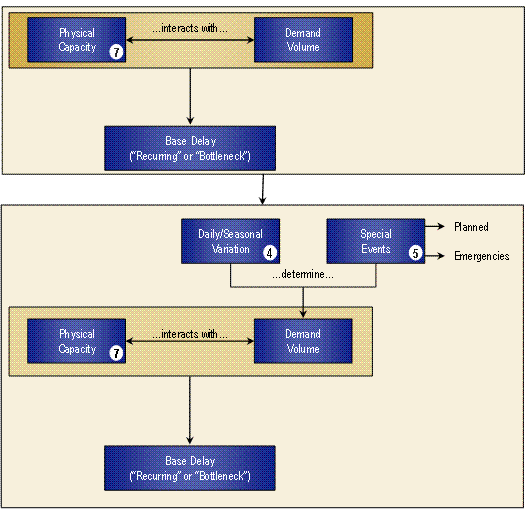
= Source of Congestion

Notation: The starting bespeak for congestion on almost days is the amount of traffic and the physical restrictions on the highway (bottlenecks). Traffic varies from day-to-solar day throughout the yr and special events may cause surges in traffic at unexpected times. See Figure 2.ii as an example of how much traffic varies even over as short a period equally a month.

Figure ii.three Anatomy of Congestion (continued)
Figure 2.3b Part 2 - Roadway Events Reduce Bachelor Capacity and Add Actress Filibuster to the System

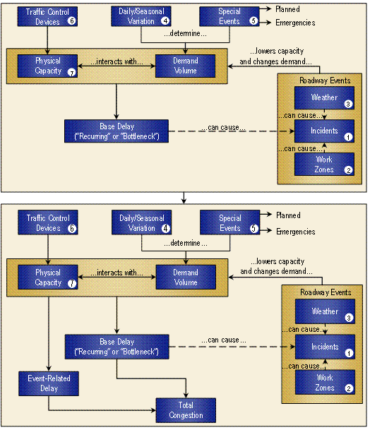
= Source of Congestion

Annotation: Just as traffic varies across time periods, so does physical capacity. The operation of traffic signals changes capacity, ofttimes infinitesimal-to-minute. When roadway events occur, they as well cause the physical capacity of the roadway to exist lowered. (Traffic incidents and work zones can "steal" lanes, and bad weather causes drivers to space themselves out more.) Base-level congestion caused by bottlenecks tin can lead to increased traffic incidents due to tighter vehicle spacing and vehicles overheating in summer. Finally, the being of extreme congestion can crusade some drivers to change their routes or to forego trips altogether. Understanding how all these factors interact is the subject of ongoing research.

Figure 2.four Relationship of Incident and Bottleneck Delay to Traffic Intensity

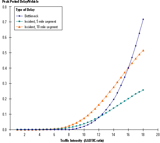
Note: The AADT/C level is a general indicator of the "intensity" of traffic trying to employ a highway with fixed chapters. AADT is Almanac Average Daily Traffic (vehicles per day) and C is the 2-way capacity of the roadway (vehicles per hour). Clogging and traffic incident delay occur differently: bottlenecks cause delay at specific points while traffic incidents may occur anywhere forth a highway segment. This is the reason for using 5- and 10-mile segments for the traffic incident delay above. The assay shows that every bit traffic grows on a roadway with fixed capacity, traffic incident filibuster is initially higher than bottleneck delay. As traffic grows, bottleneck delay overtakes traffic incident delay, considering information technology happens fairly regularly while traffic incidents vary in occurrence and characteristics.

This analysis also shows the interrelationship between the sources of delay identified in Figures 2.3a and ii.3b. Even with no changes in traffic incident characteristics, traffic incident filibuster grows equally more than traffic is added to a roadway. In other words, every bit the traffic level grows on a base of operations of stock-still chapters, the roadway is more vulnerable to disruptions caused by traffic incidents, or any other traffic-influencing effect for that matter.

The exponential growth in bottleneck delay after the onset of congestion is a major reason why it is so hard for agencies to go along up with congestion: once it starts, things go bad quickly. Introducing an actress vehicle to congested conditions means not only does that vehicle get delayed, it also adds actress delay to any other vehicles that bring together after it.

• At higher base congestion levels, clogging-related congestion grows at an increasingly faster rate. Researchers accept long noted that delay increases exponentially (i.eastward., it goes "ballistic") with traffic level on a fixed capacity base of operations. Why is this? Once a queue has formed and an additional vehicle joins at the back of the queue, you get a double whammy: not only is that vehicle delayed, just the queue is now longer and any new vehicles that bring together in will also be delayed past the now longer queue. The growth in delay for traffic incidents is more than of a straight line, the results of the irregular occurrence of traffic incidents—they practise not happen consistently like bottleneck delay does.

The fact that both bottleneck- and incident-related delay increase with base of operations congestion level indicates that if physical chapters is increased, congestion for both sources would exist decreased. In other words, Facilities with greater base capacity are less vulnerable to disruptions: a traffic incident that blocks a single lane has a greater impact on a highway with ii travel lanes than a highway with three travel lanes. This feature highlights the interdependence of the sources mentioned above. It also reinforces the notion that adding physical capacity is a viable choice for improving congestion, especially when made in conjunction with other strategies.

2.two.3 The Reliability of Travel Fourth dimension and Why It Matters

What Is Travel Time Reliability? By its very nature, roadway operation is at the same time consistent and repetitive, and yet highly variable and unpredictable. It is consequent and repetitive in that peak usage periods occur regularly and tin be predicted with a loftier degree of reliability. (The relative size and timing of "rush hour" is well known in well-nigh communities.) At the same time, it is highly variable and unpredictable, in that on any given twenty-four hours, unusual circumstances such equally crashes can dramatically modify the performance of the roadway, affecting both travel speeds and throughput volumes.

The traveling public experiences these large performance swings, and their expectation or fear of unreliable traffic conditions affects both their view of roadway performance, and how and when they choose to travel. For instance, if a road is known to have highly variable traffic atmospheric condition, a traveler using that road to grab an airplane routinely leaves lots of "extra" fourth dimension to go to the airdrome. In other words, the "reliability" of this traveler's trip is directly related to the variability in the performance of the road she or he takes.

It is condign articulate that nosotros can no longer just define congestion in terms of "average" or "typical" conditions. 1 of the reasons was identified in Figure 2.4—equally the traffic on a fixed capacity roadway, a highway becomes more susceptible to delay from traffic incidents, and in fact, to all traffic-influencing events. Because reliability indicates how much events influence traffic conditions, it is peculiarly important when it comes to defining operations strategies, which aim to control the effect of these events.

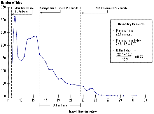
Highlight Box 2 – Measuring Reliability

Because reliability is defined by how travel times vary over time, information technology is useful to develop frequency distributions to see how much variability exists. Calculating the boilerplate travel time and the size of the "buffer"—the extra time needed by travelers to ensure a high charge per unit of on-time arrival—so helps usa to develop a variety of reliability measures. These measures include the Buffer Index, the Planning Time, and the Planning Time Alphabetize (see Figure 2.5). They are all based on the same underlying distribution of travel times, but describe reliability in slightly different means:

• Planning Time – The sheer size of the buffer (the 95th percentile travel time).
• Planning Time Index – How much larger the buffer is than the "ideal" or "free menstruation" travel time (the ratio of the 95th percentile to the platonic). In the 11.five-mile long corridor shown, the ideal travel time is 11.5 minutes, bold that vehicles volition travel at 60 mph when no congestion is nowadays.
• Buffer Index – The size of the buffer as a percent of the average (95th percentile minus the boilerplate, divided past the average.

 

Figure two.5 Distribution of Travel Times, State Route 520 Seattle, Eastbound, 4:00-7:00 p.1000. Weekdays (11.five Miles Long)

With this discussion in mind, from a practical standpoint, travel time reliability can be defined in terms of how travel times vary over time (due east.g., hour-to-hour, solar day-to-day). Commuters who take congested highways to and from piece of work are well aware of this. When asked about their commutes, they will say things similar: "information technology takes me 45 minutes on a good twenty-four hour period, just an hour and 15 minutes on a bad twenty-four hour period."

Effigy 2.6 typifies this experience with data from Land Route (SR) 520, a major commuter route, in Seattle, Washington. If there was no congestion on this 11.5 mile segment, travel times would be around eleven 1/two minutes; on President'south 24-hour interval this was the case. On other days, the average travel time was 17.5 minutes, or an boilerplate speed of 40 mph. But when events (traffic incidents and conditions) are present, it could take nearly 25 minutes, or 37 percent longer. Commuters who accept SR 520 corridor must plan for this unpredictable variability if they want to go far on time—the average just will not do.

Figure two.6 Weekday Travel Times
five:00-6:00 p.yard., on Land Route 520 Eastbound, Seattle, Washington

In other words, they accept to build in a buffer to their trip planning to account for the variability. If they build in a buffer, they will arrive early on some days, which is not necessarily a bad thing, only the extra fourth dimension is nevertheless carved out of their solar day. And this is fourth dimension they could be using for other pursuits besides commuting.

What Value Does Providing Reliable Travel Times Have? Improving the reliability of travel times is pregnant for a number of reasons:

• Improvements in reliability are accomplished by lessening the overall variability due to the 7 sources of congestion, mainly traffic-influencing events. In other words, comeback strategies targeted at reliability subtract the filibuster due to traffic-influencing events (e.g., traffic incidents, bad weather, and piece of work zones). This produces a double benefit: not merely is variability reduced but the total congestion delay experienced by travelers is also reduced.
• Reducing total congestion saves time and fuel, and leads to decreased vehicle emissions.
• Reducing congestion at international border crossings leads to lower transportation costs and benefits the national economic system every bit a whole. Farther, reducing congestion on United States highways for freight moving between Canada and Mexico fosters international trade. Therefore, congestion on U.s.a. highways has a large influence on the efficiency of international trade .
• Treating three major components of unreliable travel—traffic incidents, bad weather, and work zones—also leads to safer highways. By reducing the elapsing of these events, nosotros are reducing how long travelers are exposed to less safe weather condition.
• Commuters as well as freight carriers and shippers are all concerned with travel time reliability. Variations in travel time can be highly frustrating and are valued highly by both groups. Previous research^viii indicates that commuters value the variable component of their travel time betwixt one and six times as much as average travel fourth dimension. And the increase in just-in-time (JIT) manufacturing processes has made a reliable travel time extremely of import. Significant variations in travel time will decrease the benefits that come from lower inventory space and the apply of efficient transportation networks as "the new warehouse." Therefore, in both the passenger and freight realms, evidence suggests that travel time reliability is valued at a significant "premium" past users.

ii.2.4 How Travelers, Operators, and Planners View Reliability

Despite our simple definition of travel time reliability as the variation in travel times over history, different perspectives exist:

• Travelers want to know information near the specific trip they are about to brand and how it compares to their typical or expected trip;
• Similarly, operators desire to know how the organisation is performing now in relation to typical conditions; and
• Planners want to know how the organisation performed last month or terminal year in comparison to previous fourth dimension periods.

As we have already seen, some days are better (or worse) than others in terms of congestion, and in that location is quite a bit of variation from boilerplate or typical weather on whatever given day. Effigy 2.7 displays this variation from the traveler and operator points of view. Shown are travel times in the heavily congested I 75 corridor in central Atlanta for all Thursdays in 2003. The boilerplate and 95th percentile travel times are shown along with the bodily travel times from two specific Thursdays. January sixteen was conspicuously a "bad" mean solar day in this corridor while September iv was "better than average." For both travelers and operators, a constantly updated display of travel conditions compared to baselines would be valuable information to have. In fact, at least one traffic management eye (Houston TRANSTAR) posts this sort of data on their spider web site in real-time.⁹ Information technology should be noted that currently nosotros do non have the ability to predict what is going to happen—a difficult task given the uncertainty of unpredictable events like incidents or sudden, intense atmospheric condition. We can only compare what is happening now to historical weather condition, but research is currently underway on this topic.

Still, the ability to predict with some certainty what travel time volition be in the about time to come is of smashing involvement to operators and travelers. Why is this important? If a driver has a routine activity that must occur every day—such every bit picking up children from mean solar day intendance—they must program on an extra amount of trip time just to be certain they practise not arrive belatedly. The same goes for local trucking firms engaged in pickup and commitment of goods. Looking again at the data in Figure 2.vii, if a traveler starts in the corridor at 5:30 p.m., on the average Thursday the trip will take virtually 12 minutes. Simply history has shown that to exist safe, they accept to plan for about 18 minutes (50 percent more) to accept merely a pocket-size risk of arriving late; they take to build in a buffer . These are non huge numbers—but this is a short corridor (four miles). The difference is, even so, a large percentage. If like weather condition exist over the rest of the commute, then the extra time starts to add together upwardly speedily. With this simple approach, an extreme outcome can cause great problems for an individual trip, but at least we tin compute a reasonable probability of arriving on time.

Figure 2.7 Is It a Good Day or Bad Solar day for Commuting: Comparing Electric current Travel Times to Historical Conditions
I-75 Southbound Primal Atlanta, Thursdays, 2003

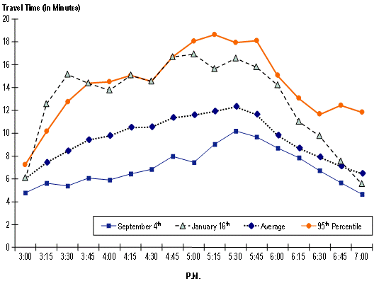
Notation: Comparing what is happening on the highway system right now to "typical" (average) and "extreme" (95th percentile) conditions provides both operators and travelers with information that tin can lead to deportment. For case, the afternoon of September iv, travelers could come across that congestion was lighter than usual and could schedule additional activities. January 16 on the other manus was a heavy congestion day and as information technology unfolded, operators could post diversion letters to try to control it.

Planners are most interested in how things change over a longer period of time, though the question of "are things getting better or worse" is of general interest besides. In the I 75 corridor in central Atlanta, travel times in the afternoon meridian period have increased and reliability has decreased between 2001 and 2003 (Figure 2.eight). Monitoring of functioning trends like this is condign more mutual at transportation agencies. As discussed in the next department, performance monitoring is a major emphasis in operations and planning.

Figure 2.8 Congestion and Unreliable Travel Accept Increased on I-75 Southbound in Central Atlanta, Georgia
Thursdays, 2001 and 2003

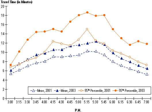
Note: Past comparison the average travel times in 2001 and 2003 (the blue lines)), it tin be seen that boilerplate congestion levels take increased in this corridor. At the aforementioned time, travel time reliability has decreased, equally shown by the increase in the 95th percentile travel times.

2.3 TRACKING CONGESTION

ii.3.1 Why Monitor Congestion?

Monitoring congestion is merely one of the several aspects of transportation organisation functioning that leads to more constructive investment decisions for transportation improvements. Safety, physical condition, environmental quality, economic development, quality of life, and client satisfaction are among the aspects of performance that also crave monitoring.¹⁰ Congestion is intertwined with all of these other categories since higher congestion levels have been associated with their degradation.

In improver to facilitating better investments, improved monitoring of congestion can lead to several positive outcomes:

• Improved Performance –The information from operating systems tin be used past the operating agencies to modify hours or methods of operation to meliorate the system. Performance measures can target, for example, before/ subsequently furnishings of recent programs or the amount of productivity lost from congested weather.
• Improved Communication – Performance measures that include travel fourth dimension, delay, or other hands understood concepts can provide better means to communicate system conditions.
• Program Justification – Functioning measures and a before/after information drove plan can be very effective at identifying the effect of a range of freeway and arterial management actions. Many of these deportment cannot be easily assessed using models.
• Funding Enhancements – In most contempo campaigns for funding increases, pricing projects or increased funding flexibility, performance measures take played two key roles. They can be used to demonstrate improved conditions or use of existing funds to show that current agency actions are appropriate and beneficial. The measures and data also can be used in public accountability pledges to demonstrate the effect of the proposed programs.

2.3.2 Congestion Performance Measures

Travel Time every bit the Basis for Congestion Performance Measures

The performance of the highway system in terms of how efficiently users can traverse it may be described in three basic terms: congestion, mobility, and accessibility. While researchers have different definitions of these terms, nosotros have plant it useful to define them as follows:

• Congestion – Describes the travel weather condition on facilities;
• Mobility – Describes how well users can complete entire trips; and
• Accessibility – Describes how close opportunities (east.thou., jobs, shopping) are spaced in terms of the user's ability to access them through the transportation system.

Congestion and mobility are very closely related and the same metrics and concepts can be used to monitor both. Accessibility is a relatively new concept and requires a unlike set of metrics. Near the information that are currently available describe facility performance, non trip performance, although new technologies are emerging that volition allow for direct monitoring of entire trips.

I of the principles that FHWA has established for monitoring congestion every bit function of its annual performance plan is that meaningful congestion performance measures must be based on the measurement of travel time. Travel times are easily understood by practitioners and the public, and are applicative to both the user and facility perspectives of operation.

Temporal Aspects of Congestion: Measuring congestion past times of the day and day of calendar week has a long history in transportation. A relatively new twist on this is the definition of a weekday "summit flow"—multiple hours rather than the traditional peak hr. In many metropolitan areas, particularly the larger ones, congestion now lasts iii or more hours each weekday morning and evening. In other words, over time, congestion has spread into more hours of the twenty-four hours as commuters go out earlier or afterwards to avoid the traditional rush hour. Definition of peak periods is critical in performing comparisons. For example, consider a three-60 minutes superlative flow. In smaller cities, congestion may unremarkably only final for i hour—better weather condition in the remaining two hours will "dilute" the metrics. Ane way around this is not to establish a fixed time menses in which to mensurate congestion, simply rather determine how long congestion exists (e.yard., percent of fourth dimension where operating conditions are below a threshold.)

Spatial Aspects of Congestion: Congestion spreads not only in time only in space as well. Queues from concrete bottlenecks and major traffic-influencing events (like traffic incidents) tin can extend for many miles. Congestion measures need to exist sensitive to this by tracking congestion over facilities or corridors, rather than just short highway segments.

Table two.two presents a small sample of congestion performance measures (metrics) that can be used by agencies to monitor trends.

Table 2.ii Case Congestion Performance Metrics

Performance Metric	Definition/Comments
Throughput
Vehicle-Miles of Travel Truck Vehicle-Miles of Travel Person-Miles of Travel	Vehicle-miles of travel are the number of vehicles on the system times the length of highway they travel. Person-miles of travel is used to accommodate for the fact that some vehicles carry more a driver.
Average Congestion Conditions
Average Travel Speed	The average speed of vehicles measured between 2 points.
Travel Time	The time it takes for vehicles to travel between ii points. Both travel time and average travel speed are adept measures for specific trips or within a corridor.
Number and percent of trips with travel times > (ane.five * average travel fourth dimension) Number and pct of trips with travel times > (2.0 * average travel fourth dimension)	Thresholds of 1.5 and two.0 times the average may exist adjusted to local conditions; additional thresholds may also be defined.
Travel Time Index	Ratio of actual travel time to an platonic (gratis-flow) travel time. Gratis-flow weather condition on freeways are travel times at a speed of 60 mph.
Total Filibuster (vehicle-hours and person-hours) Clogging ("Recurring") Delay (vehicle-hours) Traffic incident Filibuster (vehicle-hours) Work Zone Filibuster (vehicle-hours) Weather Delay (vehicle-hours) Ramp delay (vehicle-hours and person-hours; where ramp metering exists) Filibuster per Person Filibuster per Vehicle	Delay is the number of hours spent in traffic beyond what would normally occur if travel could be done at the platonic speed. Determining filibuster by "source of congestion" requires detailed information on the nature and extent of events (incidents, weather, and work zones) as well as measured travel conditions. Delay per person and delay per vehicle require knowledge of how many vehicles and persons are using the roadway.
Pct of VMT with Average Speeds < 45 mph Percent of VMT with Average Speeds < 30 mph	VMT is vehicle-miles of travel, a common measure of highway usage.
Pct of Twenty-four hour period with Average Speeds < 45 mph Pct of Solar day with Average Speeds < 30 mph	These measures capture the duration of congestion.
Reliability
Planning Time (computed for actual travel time and the Travel Time Index)	The 95th percentile of a distribution is the number to a higher place which just 5 pct of the total distribution remains. That is, only five percent of the observations exceed the 95th percentile. For commuters, this means that for 19 out of 20 workdays in a month, their trips will take no more than the Planning Fourth dimension.
Planning Time Index (computed for bodily travel fourth dimension and the Travel Time Index)	Ratio of the 95th percentile ("Planning Time") to the "ideal" or "free catamenia" travel fourth dimension (the travel time that occurs when very light traffic is nowadays, about 60 mph on near freeways).
Buffer Index	Represents the extra time (buffer) most travelers add together to their boilerplate travel time when planning trips.
For a specific road section and time menstruation: Buffer Index (%) =	95th percentile travel fourth dimension (minutes) - average travel time (minutes) boilerplate travel time (minutes)

two.3.3 Methods Used to Develop Congestion Performance Measures

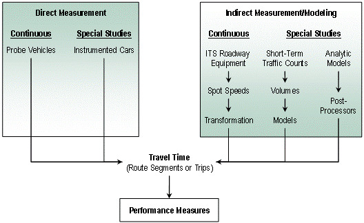
Figure ii.nine shows how travel times can be developed from data, analytic methods, or a combination. Conspicuously, the best methods are based on direct measurement of travel times, either through probe vehicles or the more traditional "floating car" method, in which data collectors drive specific routes. However, both of these accept drawbacks: probe vehicles currently are not widely deployed and the floating motorcar method suffers from extremely modest samples because it is expensive and time consuming. Further, since many performance measures require traffic volumes as well, additional collection try is required to develop the full suite of performance measures. Use of ITS roadway equipment addresses these issues, simply this equipment does not mensurate travel time straight; ITS spot speeds must be converted to travel times first. (The Appendix provides a description of the equipment used to collect these data.) Other indirect methods of travel time estimation use traffic volumes equally a basis, either those that are directly measured or developed with travel demand forecasting models. Two examples of how FHWA is developing travel times with these methods follow.

Effigy 2.9 Measuring Travel Time Is the Basis for Congestion Measures

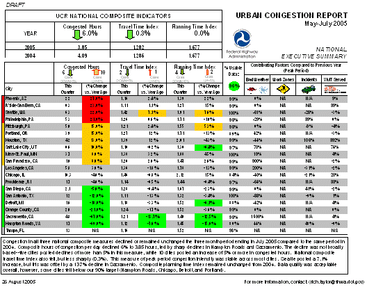
Monthly Urban Congestion Report

Since 2000, FHWA has been assembling volume and speed data from urban traffic management centers. These information are primarily from ITS roadway equipment, although some cities are exploring the employ of probe vehicles to capture travel fourth dimension. Information from 29 cities are currently obtained annually from participating traffic direction centers. Some of these cities are now providing information on a monthly basis, and these monthly data are used to rail citywide trends month-by-month. Figure 2.10 shows an example of how these information are presented. As more than cities participate—and equally surveillance coverage increases in existing cities—these information will provide a way for FHWA to monitor monthly changes in congestion. (Department 3.0 presents additional analysis of the information used in this program.)

Figure 2.x Instance of the Newly Designed Urban Congestion Study Used past FHWA to Track Monthly Changes in Congestion

Freight Performance Measurement Initiative

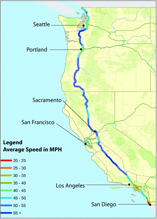
The tracking of congestion inside cities is dependent on having an intensive system of surveillance to collect vehicle speeds (through roadway detectors) or travel times (using toll-tagged probe vehicles) at closely spaced points on the roadway. Exterior of major metropolitan areas, such surveillance does non exist. To complement urban congestion measures and become a better picture of full system performance, FHWA is developing a system to monitor truck travel on intercity corridors that have significant freight volumes. FHWA is partnering with the American Transportation Inquiry Institute and the trucking industry to use existing satellite-based systems that track truck movement for freight and fleet management purposes to support transport organization performance measurement. Additionally, FHWA is exploring using similar methods to measure delay at major international edge crossings. Figure 2.11 shows an example of how this system has been practical to develop travel times on x-mile stretches of Interstate 5.

Figure two.11 Interstate 5 Average Travel Charge per unit for Trucks: ten-Mile Segments
April-June 2004, 3:00-vii:00 p.g.

2.4 CONGESTION'South CONSEQUENCES

The nation's local, regional, and national transportation systems play a vital role in creating admission to appurtenances and services which sustain and grow our nation'south economy. Planners and economic development experts recognize that congestion is an economical development issue considering information technology thwarts business attraction and expansion, and reduces the quality of life for residents.

Transportation system users have adult strategies to deal with increased congestion and reduced reliability. In the short term, we might alter our mode or fourth dimension of travel. Over the longer run, congestion might influence our decisions almost where we alive and work. The aforementioned holds truthful for businesses. These types of adjustments might reduce the impacts of congestion to united states, simply they still exercise not entirely eliminate the economic consequences for a region.

Trucking Impacts. Congestion means longer travel times and less reliable selection-up and delivery times for truck operators. To recoup, motor carriers typically add vehicles and drivers and extend their hours of functioning, eventually passing the extra costs forth to shippers and consumers. Research on the trucking industry has shown that shippers and carriers value transit fourth dimension in the range of $25 to $200 per hour, depending on the product being carried. The price of unexpected delay can add together some other 20 percent to 250 per centum.¹¹

Impacts on Businesses. Congestion increases the costs of delivering appurtenances and services, considering of the increased travel times and operating costs incurred on the transportation arrangement. Less patently, there may be are other costs, such equally:

• The costs of remaining open up for longer hours to process belatedly deliveries;
• Penalties or lost business organisation acquirement associated with missed schedules;
• Costs of spoilage for time-sensitive, perishable deliveries;
• Costs of maintaining greater inventory to cover the undependability of deliveries;
• Costs of reverting to less efficient production scheduling processes; and
• The additional costs incurred considering of access to reduced markets for labor, customer, and delivery areas.

The business value of time filibuster and market access act together to bear upon the profitability and revenue potential associated with doing business in a state or region. When one area is afflicted by congestion more than others, the relative competitiveness of these areas besides shifts. The event, then, is that businesses tend to stagnate or move out of areas with loftier operating costs and limited markets, while they locate and expand in areas with lower operating costs and broader market connections. The magnitude of these changes varies by manufacture, based on how strongly the industry'south total operating cost is afflicted past transportation factors. The evidence seems to indicate that regional economies that are fostered by clusters or "agglomerations" of many interrelated firms are better positioned to counter the higher operating costs due to congestion than economies that are not.

Household Impacts. Households accept both financial budgets and what is termed "time budgets" that are both impacted past congestion. Households plan their activities effectually the available time budget as well as around their financial budgets. As vehicle operating and maintenance costs increase with ascent congestion, the upkeep for some types of activities or expenditures decreases. The perceived "quality of life" of a neighborhood is diminished every bit well, when the safety, reliability and the convenience of the transportation system decreases.

Regional Impacts. Regional economies are affected by these household and business-specific impacts. Diminished cost competitiveness and market place growth opportunities are tantamount to a reduced ability to retain, grow, and attract businesses. Additionally, the redistribution of business concern and household action to outlying areas and the directly delay for trips that are non diverted or otherwise changed both lead to decreases in air quality, increases in public infrastructure investment requirements, and potential impacts on health and quality of life factors.¹²

---

5. Providing a Highway System with Reliable Travel Times, Time to come Strategic Highway Research Programme Expanse 3, Transportation Enquiry Lath, September 2003, http://www4.trb.org/ trb/newshrp.nsf/spider web/progress_reports?OpenDocument.
6. This phenomenon is sometimes referred to as "secondary crashes"—crashes that would non have occurred unless an earlier one in close proximity occurred. Possible causes of secondary crashes include rapidly growing queues caused by the first crash and rubbernecking by motorists.
7. Average Annual Daily Traffic – the amount of traffic that moves on the average day. Computed as simple average of all 24-hour traffic throughout the year. The AADT-to-capacity ratio is similar to the volume-to-capacity used in many transportation analyses, except the former uses 24-hour total traffic while the later on uses hourly traffic.
8. Cohen, Harry, and Southworth, Frank, On the Measurement and Valuation of Travel Time Variability Due to Incidents on Freeways, Journal of Transportation Statistics, Volume 2, Number 2, December 1999, http://www.bts.gov/jts/V2N2/vol2_n2_toc.html.
9. http://traffic.houstontranstar.org/layers/.
10. More detail on monitoring comprehensive transportation organization functioning may be found in: A Guidebook for Functioning-Based Transportation Planning, NCHRP Written report 446, Transportation Research Board, Washington, D.C., 2000.
11. Federal Highway Assistants, Freight Transportation: Improvements and the Economy; https://ops.fhwa.dot.gov/freight/freight_analysis/improve_econ/.
12. Weisbrod, Glen, Vary, Don, and Treyz, George, Economic Implications of Congestion, NCHRP Report 463, Transportation research Lath, 2001.

Dorsum to Top

Previous | Tabular array of Contents | Next

fewfourpried85.blogspot.com

Source: https://ops.fhwa.dot.gov/congestion_report/chapter2.htm

Share this post